Computable number

In mathematics, particularly theoretical computer science and mathematical logic, the computable numbers, also known as the recursive numbers or the computable reals, are the real numbers that can be computed to within any desired precision by a finite, terminating algorithm. Equivalent definitions can be given using μ-recursive functions, Turing machines or λ-calculus as the formal representation of algorithms. The computable numbers form a real closed field and can be used in the place of real numbers for many, but not all, mathematical purposes.

1 Informal definition using a Turing machine as example
2 Formal definition
3 Properties
4 Digit strings and the Cantor and Baire spaces
5 Can computable numbers be used instead of the reals?
6 Implementation
7 See also
8 References

Informal definition using a Turing machine as example

In the following, Marvin Minsky defines the numbers to be computed in a manner similar to those defined by Alan Turing in 1936, i.e. as "sequences of digits interpreted as decimal fractions" between 0 and 1:

"A computable number [is] one for which there is a Turing machine which, given n on its initial tape, terminates with the nth digit of that number [encoded on its tape]." (Minsky 1967:159)

The key notions in the definition are (1) that some n is specified at the start, (2) for any n the computation only takes a finite number of steps, after which the machine produces the desired output and terminates.

An alternate form of (2) – the machine successively prints all n of the digits on its tape, halting after printing the n^th – emphasizes Minsky's observation: (3) That by use of a Turing machine, a finite definition – in the form of the machine's table – is being used to define what is a potentially-infinite string of decimal digits.

This is however not the modern definition which only requires the result be accurate to within any given accuracy. The informal definition above is subject to a rounding problem called the table-maker's dilemma whereas the modern definition is not.

Formal definition

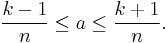
A real number a is said to be computable if it can be approximated by some computable function in the following manner: given any integer $n \ge 1$ , the function produces an integer k such that:

${k-1\over n} \leq a \leq {k%2B1\over n}.$

There are two similar definitions that are equivalent:

There exists a computable function which, given any positive rational error bound $\varepsilon$ , produces a rational number r such that $|r - a| \leq \varepsilon.$
There is a computable sequence of rational numbers $q_i$ converging to $a$ such that $|q_i - q_{i%2B1}| < 2^{-i}\,$ for each i.

There is another equivalent definition of computable numbers via computable Dedekind cuts. A computable Dedekind cut is a computable function $D\;$ which when provided with a rational number $r$ as input returns $D(r)=\mathrm{true}\;$ or $D(r)=\mathrm{false}\;$ , satisfying the following conditions:

$\exists r D(r)=\mathrm{true}\;$

$\exists r D(r)=\mathrm{false}\;$

$(D(r)=\mathrm{true}) \wedge (D(s)=\mathrm{false}) \Rightarrow r<s\;$

$D(r)=\mathrm{true} \Rightarrow \exist s>r, D(s)=\mathrm{true}.\;$

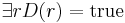
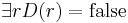
An example is given by a program D that defines the cube root of 3. Assuming $q>0\;$ this is defined by:

$p^3<3 q^3 \Rightarrow D(p/q)=\mathrm{true}\;$

$p^3>3 q^3 \Rightarrow D(p/q)=\mathrm{false}.\;$

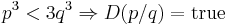
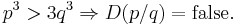
A real number is computable if and only if there is a computable Dedekind cut D converging to it. The function D is unique for each irrational computable number (although of course two different programs may provide the same function).

A complex number is called computable if its real and imaginary parts are computable.

Properties

While the set of real numbers is uncountable, the set of computable numbers is only countable and thus almost all real numbers are not computable. The computable numbers can be counted by assigning a Gödel number to each Turing machine definition. This gives a function from the naturals to the computable reals. Although the computable numbers are an ordered field, the set of Gödel numbers corresponding to computable numbers is not itself computably enumerable, because it is not possible to effectively determine which Gödel numbers correspond to Turing machines that produce computable reals. In order to produce a computable real, a Turing machine must compute a total function, but the corresponding decision problem is in Turing degree 0′′. Thus Cantor's diagonal argument cannot be used to produce uncountably many computable reals; at best, the reals formed from this method will be uncomputable.

The arithmetical operations on computable numbers are themselves computable in the sense that whenever real numbers a and b are computable then the following real numbers are also computable: a + b, a - b, ab, and a/b if b is nonzero. These operations are actually uniformly computable; for example, there is a Turing machine which on input (A,B, $\epsilon$ ) produces output r, where A is the description of a Turing machine approximating a, B is the description of a Turing machine approximating b, and r is an $\epsilon$ approximation of a+b.

The computable real numbers do not share all the properties of the real numbers used in analysis. For example, the least upper bound of a bounded increasing computable sequence of computable real numbers need not be a computable real number (Bridges and Richman, 1987:58). A sequence with this property is known as a Specker sequence, as the first construction is due to E. Specker (1949). Despite the existence of counterexamples such as these, parts of calculus and real analysis can be developed in the field of computable numbers, leading to the study of computable analysis.

The order relation on the computable numbers is not computable. There is no Turing machine which on input A (the description of a Turing machine approximating the number $a$ ) outputs "YES" if $a > 0$ and "NO" if $a \le 0$ . The reason: suppose the machine described by A keeps outputting 0 as $\epsilon$ approximations. It is not clear how long to wait before deciding that the machine will never output an approximation which forces a to be positive. Thus the machine will eventually have to guess that the number will equal 0, in order to produce an output; the sequence may later become different from 0. This idea can be used to show that the machine is incorrect on some sequences if it computes a total function. A similar problem occurs when the computable reals are represented as Dedekind cuts. The same holds for the equality relation : the equality test is not computable.

While the full order relation is not computable, the restriction of it to pairs of unequal numbers is computable. That is, there is a program that takes an input two turing machines A and B approximating numbers a and b, where a≠b, and outputs whether a<b or a>b. It is sufficient to use ε-approximations where ε<|b-a|/2; so by taking increasingly small ε (with a limit to 0), one eventually can decide whether a<b or a>b.

Every computable number is definable, but not vice versa. There are many definable, noncomputable real numbers, including:

The binary representation of the Halting problem (or any other uncomputable set of natural numbers).
Chaitin's constant, $\Omega$ , which is a type of real number that is Turing equivalent to the Halting problem.

A real number is computable if and only if the set of natural numbers it represents (when written in binary and viewed as a characteristic function) is computable.

Every computable number is arithmetical.

The set of computable real numbers (as well as every countable, densely ordered subset of reals without ends) is order-isomorphic to the set of rational numbers.

Digit strings and the Cantor and Baire spaces

Turing's original paper defined computable numbers as follows:

A real number is computable if its digit sequence can be produced by some algorithm or Turing machine. The algorithm takes an integer $n \ge 1$ as input and produces the $n$ -th digit of the real number's decimal expansion as output.

(Note that the decimal expansion of a only refers to the digits following the decimal point.)

Turing was aware that this definition is equivalent to the $\epsilon$ -approximation definition given above. The argument proceeds as follows: if a number is computable in the Turing sense, then it is also computable in the $\epsilon$ sense: if $n > \log_{10} (1/\epsilon)$ , then the first n digits of the decimal expansion for a provide an $\epsilon$ approximation of a. For the converse, we pick an $\epsilon$ computable real number a and generate increasingly precisce approximations until the nth digit after the decimal point is certain. This always generates a decimal expansion equal to a but it may improperly end in an infinite sequence of 9's in which case it must have a finite (and thus computable) proper decimal expansion.

Unless certain topological properties of the real numbers are relevant it is often more convenient to deal with elements of $2^{\omega}$ (total 0,1 valued functions) instead of reals numbers in $[0,1]$ . The members of $2^{\omega}$ can be identified with binary decimal expansions but since the decimal expansions $.d_1d_2\ldots d_n0111\ldots$ and $.d_1d_2\ldots d_n10$ denote the same real number the inteveral $[0,1]$ can only be bijectively (and homeomorphically under the subset topology) identified with the subset of $2^{\omega}$ not ending in all 1's.

Note that this property of decimal expansions means it's impossible to effectively identify computable real numbers defined in terms of a decimal expansion and those defined in the $\epsilon$ approximation sense. Hirst has shown there is no algorithm which takes as input the description of a Turing machine which produces $\epsilon$ approximations for the computable number a, and produces as output a Turing machine which enumerates the digits of a in the sense of Turing's definition (see Hirst 2007). Similarly it means that the arithmetic operations on the computable reals are not effective on their decimal representations as when adding decimal numbers, in order to produce one digit it may be necessary to look arbitrarily far to the right to determine if there is a carry to the current location. This lack of uniformity is one reason that the contemporary definition of computable numbers uses $\epsilon$ approximations rather than decimal expansions.

However, from a computational or measure theoretic perspective the two structures $2^{\omega}$ and $[0,1]$ are essentially identical. and computability theorists often refer to members of $2^{\omega}$ as reals. While $[0,1]$ $2^{\omega}$ is totally disconnected for questions about $\Pi^0_1$ classes or randomness it's much less messy to work in $2^{\omega}$ .

Elements of $\omega^{\omega}$ are sometimes called reals as well and though containing a homeomorphic image of $\mathbb{R}$ $\omega^{\omega}$ in addition to being totally disconnected isn't even locally compact. This leads to genuine differences in the computational properties. For instance the $x \in \mathbb{R}$ satisfying $\forall(n \in \omega)\phi(x,n)$ with $\phi(x,n)$ quatifier free must be computable while the unique $x \in \omega^{\omega}$ satisfying a universal formula can be arbitrarily high in the hyperarithmetic hierarchy.

Can computable numbers be used instead of the reals?

The computable numbers include many of the specific real numbers which appear in practice, including all algebraic numbers, as well as e, $\pi$ , and many other transcendental numbers. Though the computable reals exhaust those reals we can calculate or approximate, the assumption that all reals are computable leads to substantially different conclusions about the real numbers. The question naturally arises of whether it is possible to dispose of the full set of reals and use computable numbers for all of mathematics. This idea is appealing from a constructivist point of view, and has been pursued by what Bishop and Richman call the Russian school of constructive mathematics.

To actually develop analysis over computable numbers, some care must be taken. For example, if one uses the classical definition of a sequence, the set of computable numbers is not closed under the basic operation of taking the supremum of a bounded sequence (for example, consider a Specker sequence). This difficulty is addressed by considering only sequences which have a computable modulus of convergence. The resulting mathematical theory is called computable analysis.

Implementation

There are some computer packages that work with computable real numbers, representing the real numbers as programs computing approximations. One example is the RealLib package (reallib home page).

References

Oliver Aberth 1968, Analysis in the Computable Number Field, Journal of the Association for Computing Machinery (JACM), vol 15, iss 2, pp 276–299. This paper describes the development of the calculus over the computable number field.
Errett Bishop and Douglas Bridges, Constructive Analysis, Springer, 1985, ISBN 0387150668
Douglas Bridges and Fred Richman. Varieties of Constructive Mathematics, Oxford, 1987.
Jeffry L. Hirst, Representations of reals in reverse mathematics, Bulletin of the Polish Academy of Sciences, Mathematics, 55, (2007) 303–316.
Marvin Minsky 1967, Computation: Finite and Infinite Machines, Prentice-Hall, Inc. Englewood Cliffs, NJ. No ISBN. Library of Congress Card Catalog No. 67-12342. His chapter §9 "The Computable Real Numbers" expands on the topics of this article.
E. Specker, "Nicht konstruktiv beweisbare Sätze der Analysis" J. Symbol. Logic, 14 (1949) pp. 145–158
Turing, A.M. (1936), "On Computable Numbers, with an Application to the Entscheidungsproblem", Proceedings of the London Mathematical Society, 2 42 (1): 230–65, 1937, doi:10.1112/plms/s2-42.1.230, http://www.abelard.org/turpap2/tp2-ie.asp (and Turing, A.M. (1938), "On Computable Numbers, with an Application to the Entscheidungsproblem: A correction", Proceedings of the London Mathematical Society, 2 43 (6): 544–6, 1937, doi:10.1112/plms/s2-43.6.544 ). Computable numbers (and Turing's a-machines) were introduced in this paper; the definition of computable numbers uses infinite decimal sequences.
Klaus Weihrauch 2000, Computable analysis, Texts in theoretical computer science, Springer, ISBN 3540668179. §1.3.2 introduces the definition by nested sequences of intervals converging to the singleton real. Other representations are discussed in §4.1.
Klaus Weihrauch, A simple introduction to computable analysis

Computable numbers were defined independently by Turing, Post and Church. See The Undecidable, ed. Martin Davis, for further original papers.

Number systems

Countable sets	Natural numbers ( $\scriptstyle\mathbb{N}$ ) Integers ( $\scriptstyle\mathbb{Z}$ ) Rational numbers ( $\scriptstyle\mathbb{Q}$ ) Algebraic numbers ( $\scriptstyle\overline{\mathbb{Q}}$ ) Periods Computable numbers Arithmetical numbers

Real numbers and their extensions	Real numbers ( $\scriptstyle\mathbb{R}$ ) Complex numbers ( $\scriptstyle\mathbb{C}$ ) Quaternions ( $\scriptstyle\mathbb{H}$ ) Octonions ( $\scriptstyle\mathbb{O}$ ) Sedenions ( $\scriptstyle\mathbb{S}$ ) Cayley–Dickson construction Dual numbers Hypercomplex numbers Superreal numbers Irrational numbers Transcendental numbers Hyperreal numbers Surreal numbers

Other number systems	Cardinal numbers Ordinal numbers p-adic numbers Supernatural numbers